Running Distributed Quality-Diversity Algorithms on HPC

Tips and tricks to avoid a world of pain.

Overview ¶

Back in September, I began learning to run Quality-Diversity (QD) algorithms on USC’s HPC. Since then, I have learned a number of lessons that may prove useful to others seeking to do the same. In short, this article covers the structure of distributed QD algorithms, the types of hardware on which they can be distributed, libraries for utilizing this hardware, and several implementation considerations. Though I focus on QD algorithms implemented in Python in this article, the lessons are applicable to other algorithms (potentially implemented in other languages) that require many expensive objective function evaluations. My hope is that others can refer to this article and avoid frustrating pitfalls when using HPC.

Contents ¶

Distributed QD Algorithms ¶

For a given problem, Quality-Diversity (QD) algorithms seek to find high-performing solutions that exhibit different properties, known as behavior characteristics. To that end, a QD algorithm typically maintains an archive of solutions it has found so far with various BCs. For $n$ generations, the QD algorithm creates new solutions based on the ones currently in the archive, evaluates those solutions, and attempts to insert them back into the archive. Here is that process in pseudo code:

archive = init_archive()

for n in range(generations):
    solutions = create_new_solutions(archive)
    evaluate(solutions)
    insert_into_archive(solutions)

For those using pyribs, the pseudocode is fairly similar:

archive = ...
emitters = ...
optimizer = Optimizer(archive, emitters)
for itr in range(total_itrs):
    solutions = optimizer.ask()
    objectives, bcs = evaluate(solutions)
    optimizer.tell(objectives, bcs)

Within the main loop, the bottleneck tends to be the evaluation of solutions. Usually, the other parts are quick: creating new solutions only involves sampling from a multivariate Gaussian distribution, ¹ Oftentimes, this distribution is diagonal, making sampling even quicker. [Close] and inserting into the archive involves doing a lookup in an array, hash map, or other fast data structure. ² For example, in the Centroidal Voronoi Tesselation (CVT) MAP-Elites algorithm, one may use a k-D tree to find the correct bin in the archive. [Close] In contrast, evaluating even a single solution can be computationally expensive. This is particularly true in RL, where a solution is the policy for an agent, and evaluation involves rolling out the policy in simulation with software like MuJoCo, Bullet, or Box2D. Fortunately, evaluations are embarrassingly parallel. Since the evaluation of one solution in a generation does not depend on the evaluation of any other solutions in that generation, it is easy to run many evaluations at the same time.

Knowing that evaluations take a long time, we can speed up our QD algorithm by distributing the evaluations. To do that, we use a layout like the following. In this layout, a main worker runs the algorithm and distributes solutions for the workers to evaluate. Once the workers finish their evaluations, they return their results back to the main worker.

Typically, each worker corresponds to a single process running on a single CPU core, though configurations vary across problem settings and languages. This means the main worker is running the rest of the entire QD algorithm (creating new solutions, inserting solutions into the archive) on a single CPU core. As such, these operations must be fast, such that they are negligible when compared to the time the workers spend on evaluations.

With this layout in mind, we can update our pseudo code. In the rest of this tutorial, we show how to put this distributed layout into practice.

archive = init_archive()

for n in range(generations):
    solutions = create_new_solutions(archive)
    distribute_evaluations(solutions)
    retrieve_evaluation_results()
    insert_into_archive(solutions)

Hardware ¶

Running a distributed QD algorithm requires powerful hardware. We will cover two options for hardware: a single machine and USC’s High-Performance Computing cluster (HPC).

Single Machine ¶

If our evaluations are not too expensive, a single multicore machine may suffice. Modern laptops contain at least 4 cores (allowing 8 concurrent threads due to hyperthreading), and if that is not enough, there are machines with even more cores, like some of the ones in the ICAROS Lab.

HPC ¶

For even more power, we turn to the High-Performance Computing (HPC) services offered by USC’s Center for Advanced Research Computing (CARC). With thousands of CPUs available across hundreds of machines, the HPC easily has more power than any reasonable single machine. However, there is some overhead in understanding how the HPC works. The following diagram shows the various components of USC’s HPC. In our work, we are mainly concerned with the Discovery login nodes (top left corner) and Discovery Cluster compute nodes (top right corner).

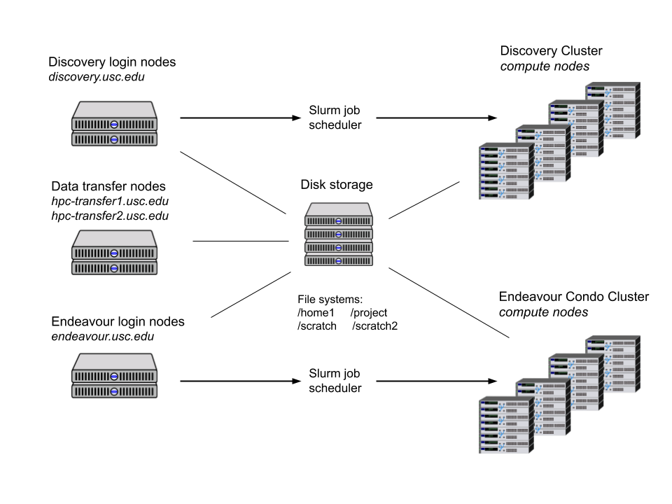
Each node on the HPC is a machine with 20+ cores and large amounts of RAM (often 100+ GB). To use these nodes, we begin by logging into the login nodes at discovery.usc.edu. Then, to run computations, we submit jobs to the Slurm scheduler, which runs the job on the compute nodes. In our distributed QD algorithm, we will submit a job that runs the main worker, and we will submit several jobs that each start multiple workers on separate machines. To make things more concrete, if we are running an algorithm with 120 workers, one way to obtain the workers would be:

• Submit 1 job for the main worker
• Submit 10 jobs that each request 12 cores (1 core per worker, so that 12 workers are in each job)

Distributing Computation with Dask ¶

Though we have the hardware, we still have to implement the algorithm, including the connections between workers. For connecting the workers, there are many distributed computation libraries available in Python, such as Ray, Fiber, and even Python’s multiprocessing module. We choose to use Dask, as we find that it has a large community and good support for a wide variety of platforms, including single machines and HPC.

Dask operates around the idea of a cluster of workers that all connect to a scheduler. To request work from the cluster, we start a script that connects to the scheduler and makes requests. The scheduler then runs the computations on the workers and returns the results. Thus, we can slightly modify the layout from earlier to look like the following, where we have separated the experiment from the scheduler.

Using Dask’s distributed library, we can set up clusters across multiple machines or even on a single machine. To do so on HPC, when we submit the worker job, we call dask-worker to set up workers on the node assigned to the job. On the job with the main worker, we call dask-scheduler to start the scheduler and then execute our experiment script. Though we separate the experiment and Dask Scheduler in the layout above, we run them on the same node for simplicity. Meanwhile, to set up a cluster on a single machine (i.e. locally), we can start the workers and scheduler directly with dask-worker and dask-scheduler directly, and run the script to connect to the scheduler. Overall, since Dask can handle cluster setup across many hardware settings, our algorithm can run in a variety of computing environments without any changes.

Integrating Dask into an Experiment ¶

With Dask in place, we need to build up the rest of the software stack and implement the algorithm. Implementing the algorithm itself is relatively simple, as we can use the various Python libraries (numpy, scipy, etc.). Since Dask can serialize almost any Python function, the algorithm just needs to pass the appropriate evaluation function to Dask with the solutions as arguments. For the rest of the stack, we need to ensure Dask runs consistently by providing two things: a standard environment and straightforward configuration.

Environments ¶

Though Dask can distribute any function, it does not distribute the dependencies required to run that function, instead assuming that the worker has the necessary libraries. Hence, different workers may use different library versions and thus evaluate solutions in different ways. To avoid this problem, we need to ensure each Dask worker (as well as the scheduler and experiment) runs in the same environment.

There are at least two methods for creating consistent environments on HPC. The first is virtual environments like Conda and Python environments. These mainly install various libraries and make them available on the system path. Such environments work great most of the time. However, since they still rely on the underlying system to some degree, they tend to struggle with libraries like MuJoCo, which require various system libraries to be installed. In such cases, it is better to use a container like Docker or Singularity, which essentially runs another operating system on top of the original system. HPC supports Singularity, but Singularity can also use Docker containers. Overall, using either an environment or container ensures that all workers use the same software.

Configuration ¶

Running an experiment should only require a single command, as it is impossible to manually start every node on the HPC. For this purpose, we can write a shell script that sends out all the Slurm jobs. Such a script requires two sets of configurations – one for the cluster (including number of nodes, number of workers per node, etc.), and one for the algorithm. I have found it useful to handle these two configurations separately by placing them in two separate files. Then, the cluster configurations are interchangeable. For faster runtime, more workers can be added, but the algorithm results should remain exactly the same. ³ Assuming randomness is properly controlled with a master seed. [Close] The cluster configuration may even be replaced with a local configuration, in order to test the algorithm on a single machine.

Running Robust Experiments ¶

Experiments do not always work perfectly. Even if the algorithm and evaluations run perfectly, experiments may still crash due to system limits. For instance, Slurm will cancel jobs that exceed their specified memory or time limit. Here we describe some features that make it possible to track down the cause of failure and even resurrect a failed experiment.

Logging and Monitoring ¶

Using Python’s logging module or even basic print statements, each worker can output various pieces of information about its internal state, including variable values and profiling metrics. Capturing this output is relatively easy. For each node, Slurm captures the standard output and standard error of all the workers on that node and places them in a single file. This does mean that all the worker outputs may mix with each other, but we can prefix each worker output with the worker’s address. For easy retrieval, the location of this file can be specified when starting the Slurm jobs. Furthermore, since HPC uses a shared filesystem among all nodes, all these files are immediately available later on (i.e. there is no need to transfer the logging outputs between nodes after the experiment).

During the experiment, we may wish to plot metrics such as runtime per iteration or QD score of the archive. A popular solution for doing so is Tensorboard, but on a system such as HPC, connecting to a Tensorboard server during an experiment is an additional complicated step. Since these metrics are almost always simple scalars, and one only needs a general idea of their trend, the easiest way to visualize them is to create text-based plots (i.e. ASCII art). After the experiment, the data from these plots may be placed into more visually appealing plots.

Reloading ¶

If an experiment exceeds memory or time limits and Slurm cancels it, it is useful to simply resume the experiment, as there is nothing wrong with its logic. To do so, we can save a “reload file,” typically in Pickle format, that contains the entire experiment state. If using pyribs, we would at least save the optimizer and the number of generations completed so far. A simple pitfall here is to directly save the reload data to the same file (such as reload.pkl) on every iteration. However, as reload data can be very large, the experiment may fail while saving the reload data. If this happens, the reload file will only be partially saved (i.e. it will be corrupted). ⁴ Yes, this was learned through painful experience. [Close] Thus, it is best to first save to a separate file (e.g. reload-tmp.pkl) and then rename this file to the actual reload file.

Conclusion ¶

When a QD algorithm requires millions of expensive objective function evaluations, it is impossible to run it on a single machine, so we turn to systems like HPC to run the algorithm in a distributed fashion. While the idea behind a distributed QD algorithm is fairly simple, the implementation can quickly become complicated. Even with a flexible library like Dask, there are still many implementation considerations to make in order to ensure consistent and reliable experiments.

For those looking to start running distributed QD algorithms, it is best to begin with a single machine. For this purpose, refer to the Lunar Lander example in pyribs, which uses Dask to distribute evaluations during a run of CMA-ME in the Lunar Lander environment. The example has basic implementations of many of the concepts described in this article. Afterwards, refer to the DQD-RL repo, which contains a full implementation that again uses pyribs but runs everything on HPC with Singularity containers.

Acknowledgements ¶

Many thanks to Stefanos Nikolaidis, for providing access to USC’s HPC. Figuring out how to use it has been quite the learning experience.

Footnotes ¶

1. Oftentimes, this distribution is diagonal, making sampling even quicker.
2. For example, in the Centroidal Voronoi Tesselation (CVT) MAP-Elites algorithm, one may use a k-D tree to find the correct bin in the archive.
3. Assuming randomness is properly controlled with a master seed.
4. Yes, this was learned through painful experience.